Blowup

The following figure illustrates the effect of blowups along a GKM subgraph (red) on the underlying graph. 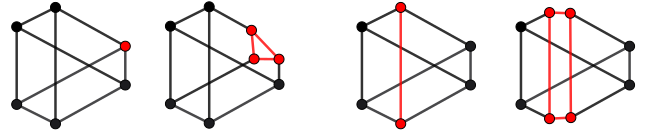Illustration of blowups along sub-GKM-graphs

Blowups of smooth and Orbifold GKM graphs

Oscar.IntersectionTheory.blowup — Function

blowup(S::AbstractGKMSubgraph)
blowup(S::AbstractGKMSubgraph, weights::AbstractVector{<:Integer})

Given a GKMSubgraph or OrbifoldGKMSubgraph structure S, return the blow up along S. An ordinary blowup of a smooth graph returns a GKMSubgraph; weighted blowups and blowups of orbifold graphs return an OrbifoldGKMSubgraph. The subgraph of the result is the exceptional divisor.

Warning

Both the blowup and the exceptional connection are equipped with the Algorithm connection.

Todo

Equip the blowup with an extension of the original connection whenever possible.

Examples of smooth blowups

julia> G = projective_space(GKMGraph, 3) # 3-dimensional projective space
GKM graph with 4 nodes, valency 3 and axial function:
2 -> 1 => (1, -1, 0, 0)
3 -> 1 => (1, 0, -1, 0)
3 -> 2 => (0, 1, -1, 0)
4 -> 1 => (1, 0, 0, -1)
4 -> 2 => (0, 1, 0, -1)
4 -> 3 => (0, 0, 1, -1)
Birkhoff-Grothendieck connection for GKM graph with 4 nodes and valency 3

julia> S = subgraph_from_vertices(G, [1, 2]) # we take the subgraph of two vertices, it corresponds to a line
GKM subgraph of:
GKM graph with 4 nodes, valency 3 and axial function:
2 -> 1 => (1, -1, 0, 0)
3 -> 1 => (1, 0, -1, 0)
3 -> 2 => (0, 1, -1, 0)
4 -> 1 => (1, 0, 0, -1)
4 -> 2 => (0, 1, 0, -1)
4 -> 3 => (0, 0, 1, -1)
Birkhoff-Grothendieck connection for GKM graph with 4 nodes and valency 3
Subgraph:
GKM graph with 2 nodes, valency 1 and axial function:
2 -> 1 => (1, -1, 0, 0)
Algorithmic connection for GKM graph with 2 nodes and valency 1

julia> blowupSub = blowup(S) # blowup of P3 along the line S
GKM subgraph of:
GKM graph with 6 nodes, valency 3 and axial function:
[1>4] -> [1>3] => (0, 0, 1, -1)
[2>3] -> [1>3] => (1, -1, 0, 0)
[2>4] -> [1>4] => (1, -1, 0, 0)
[2>4] -> [2>3] => (0, 0, 1, -1)
3 -> [1>3] => (1, 0, -1, 0)
3 -> [2>3] => (0, 1, -1, 0)
4 -> [1>4] => (1, 0, 0, -1)
4 -> [2>4] => (0, 1, 0, -1)
4 -> 3 => (0, 0, 1, -1)
Algorithmic connection for GKM graph with 6 nodes and valency 3
Subgraph:
GKM graph with 4 nodes, valency 2 and axial function:
[1>4] -> [1>3] => (0, 0, 1, -1)
[2>3] -> [1>3] => (1, -1, 0, 0)
[2>4] -> [1>4] => (1, -1, 0, 0)
[2>4] -> [2>3] => (0, 0, 1, -1)
Algorithmic connection for GKM graph with 4 nodes and valency 2

julia> Spoint = subgraph_from_vertices(G, [1]) # we take the subgraph of one vertex that is an invariant point
GKM subgraph of:
GKM graph with 4 nodes, valency 3 and axial function:
2 -> 1 => (1, -1, 0, 0)
3 -> 1 => (1, 0, -1, 0)
3 -> 2 => (0, 1, -1, 0)
4 -> 1 => (1, 0, 0, -1)
4 -> 2 => (0, 1, 0, -1)
4 -> 3 => (0, 0, 1, -1)
Birkhoff-Grothendieck connection for GKM graph with 4 nodes and valency 3
Subgraph:
GKM graph with 1 nodes, valency 0 and axial function:
Empty connection for GKM graph with 1 nodes and valency 0

julia> blowupPt = blowup(Spoint) # blowup of P3 at a point
GKM subgraph of:
GKM graph with 6 nodes, valency 3 and axial function:
[1>3] -> [1>2] => (0, 1, -1, 0)
[1>4] -> [1>2] => (0, 1, 0, -1)
[1>4] -> [1>3] => (0, 0, 1, -1)
2 -> [1>2] => (1, -1, 0, 0)
3 -> [1>3] => (1, 0, -1, 0)
3 -> 2 => (0, 1, -1, 0)
4 -> [1>4] => (1, 0, 0, -1)
4 -> 2 => (0, 1, 0, -1)
4 -> 3 => (0, 0, 1, -1)
Algorithmic connection for GKM graph with 6 nodes and valency 3
Subgraph:
GKM graph with 3 nodes, valency 2 and axial function:
[1>3] -> [1>2] => (0, 1, -1, 0)
[1>4] -> [1>2] => (0, 1, 0, -1)
[1>4] -> [1>3] => (0, 0, 1, -1)
Algorithmic connection for GKM graph with 3 nodes and valency 2

julia> ambient_blowupSub = ambient_graph(blowupSub);

julia> c3_Sub = chern_class(ambient_blowupSub, 3);

julia> integrate(c3_Sub) # we expect this to be 6
6

julia> ambient_blowupPt = ambient_graph(blowupPt);

julia> c3_Pt = chern_class(ambient_blowupPt, 3);

julia> integrate(c3_Pt) # we expect this to be 6
6

source

We can blowup also Orbifold GKM graphs.

GKMtools.weighted_blowup — Function

weighted_blowup(S::AbstractGKMSubgraph, weights::AbstractVector{<:Integer}) -> OrbifoldGKMSubgraph

See blowup.

source

An example of a blowup of an orbifold.

julia> W = stacky_weighted_projective_space_fan([1, 2, 3, 4]);

julia> Wp = gkm_graph_of_orbifold_toric(W);

julia> s = subgraph_from_vertices(Wp, [1]);

julia> GKMtools.blowup(s)
GKM subgraph of:
Orbifold GKM graph with 6 nodes, valency 3 and axial function:
[1>3] -> [1>4] => (1, -1, 0, 1)
[1>2] -> [1>4] => (1, 0, -1, 2)
[1>2] -> [1>3] => (0, 1, -1, 1)
2 -> [1>2] => (0, 0, -1, 4)
3 -> [1>3] => (0, -1, 0, 3)
3 -> 2 => (0, -4, 3, 0)
4 -> [1>4] => (-1, 0, 0, 2)
4 -> 2 => (-2, 0, 1, 0)
4 -> 3 => (-3, 2, 0, 0)
Vertex Isotropy:
2 => Orbifold Vertex Isotropy, Group Structure (cyclic factors): [4]
  Tangent Representation: 
[1   3   2]
3 => Orbifold Vertex Isotropy, Group Structure (cyclic factors): [3]
  Tangent Representation: 
[1   1   2]
4 => Orbifold Vertex Isotropy, Group Structure (cyclic factors): [2]
  Tangent Representation: 
[1   0   1]
Flag Isotropy:
2.3 => Orbifold Flag Isotropy, Group Structure (cyclic factors): [2]
  Embedding Matrix: 
[2]
4.2 => Orbifold Flag Isotropy, Group Structure (cyclic factors): [2]
  Embedding Matrix: 
[1]
Algorithmic connection for GKM graph with 6 nodes and valency 3
Subgraph:
Orbifold GKM graph with 3 nodes, valency 2 and axial function:
[1>3] -> [1>4] => (1, -1, 0, 1)
[1>2] -> [1>4] => (1, 0, -1, 2)
[1>2] -> [1>3] => (0, 1, -1, 1)
Vertex Isotropy:
Flag Isotropy:
Algorithmic connection for GKM graph with 3 nodes and valency 2

Weighted blowups

We construct the weighted blowup of the affine space $\mathbb{A}^4$ with weights weights = [1, 2, 3, 4]. We show that the result has exceptional divisor isomorphic to the weighted projective space $\mathbb{P}^3(1, 2, 3, 4)$.

julia> A4_toric = affine_space(NormalToricVariety, 4);

julia> A4_GKM = gkm_graph_of_toric(A4_toric);

julia> sub_A4 = subgraph_from_vertices(A4_GKM, [1]);

julia> blow_A4 = GKMtools.blowup(sub_A4, [1, 2, 3, 4]);

julia> subgraph(blow_A4)
Orbifold GKM graph with 4 nodes, valency 3 and axial function:
[1>F2] -> [1>F1] => (2, -1, 0, 0)
[1>F3] -> [1>F1] => (3, 0, -1, 0)
[1>F3] -> [1>F2] => (0, 3, -2, 0)
[1>F4] -> [1>F1] => (4, 0, 0, -1)
[1>F4] -> [1>F2] => (0, 2, 0, -1)
[1>F4] -> [1>F3] => (0, 0, 4, -3)
Vertex Isotropy:
[1>F2] => Orbifold Vertex Isotropy, Group Structure (cyclic factors): [2]
  Tangent Representation: 
[1   1   0]
[1>F3] => Orbifold Vertex Isotropy, Group Structure (cyclic factors): [3]
  Tangent Representation: 
[1   2   1]
[1>F4] => Orbifold Vertex Isotropy, Group Structure (cyclic factors): [4]
  Tangent Representation: 
[1   2   3]
Flag Isotropy:
[1>F2].3 => Orbifold Flag Isotropy, Group Structure (cyclic factors): [2]
  Embedding Matrix: 
[1]
[1>F4].2 => Orbifold Flag Isotropy, Group Structure (cyclic factors): [2]
  Embedding Matrix: 
[2]
Algorithmic connection for GKM graph with 4 nodes and valency 3

Let us construct the weighted projective space $\mathbb{P}^3(1, 2, 3, 4)$.

julia> W = stacky_weighted_projective_space_fan([1, 2, 3, 4]);

julia> Wp = gkm_graph_of_orbifold_toric(W)
Orbifold GKM graph with 4 nodes, valency 3 and axial function:
2 -> 1 => (0, 0, -1, 4)
3 -> 1 => (0, -1, 0, 3)
3 -> 2 => (0, -4, 3, 0)
4 -> 1 => (-1, 0, 0, 2)
4 -> 2 => (-2, 0, 1, 0)
4 -> 3 => (-3, 2, 0, 0)
Vertex Isotropy:
2 => Orbifold Vertex Isotropy, Group Structure (cyclic factors): [4]
  Tangent Representation: 
[2   3   1]
3 => Orbifold Vertex Isotropy, Group Structure (cyclic factors): [3]
  Tangent Representation: 
[2   1   1]
4 => Orbifold Vertex Isotropy, Group Structure (cyclic factors): [2]
  Tangent Representation: 
[1   0   1]
Flag Isotropy:
2.1 => Orbifold Flag Isotropy, Group Structure (cyclic factors): [2]
  Embedding Matrix: 
[2]
4.2 => Orbifold Flag Isotropy, Group Structure (cyclic factors): [2]
  Embedding Matrix: 
[1]
Algorithmic connection for GKM graph with 4 nodes and valency 3

The two constructions coincides after reodering the vertices and flags: (1, 2, 3, 4) correspond to [1>F1], [1>F4], [1>F3], [1>F2].